Network analysis
- Topics for module
- Introduction to graphs and graph theory
- Descriptive measures of graphs
- Visualizing graphs
- Generative models for network graphs
- Identifying communities
- To read: Nothing
- Slides
- R code from the exercises
Exercises
All of these exercises use the R program package. We will be needing
the igraph package, which can be installed using the
install.packages() function.
install.packages(c("igraph"))The exercises are build up over two types of problems: introductory text that you should run through to make sure you understand how to use the function(s) and interpret the output and a few additional questions for you to explore and discuss.
Creating a network and working with simple measures
In this exercise we will use the functionality of the
igraph package to create our own small network and analyze
the data.
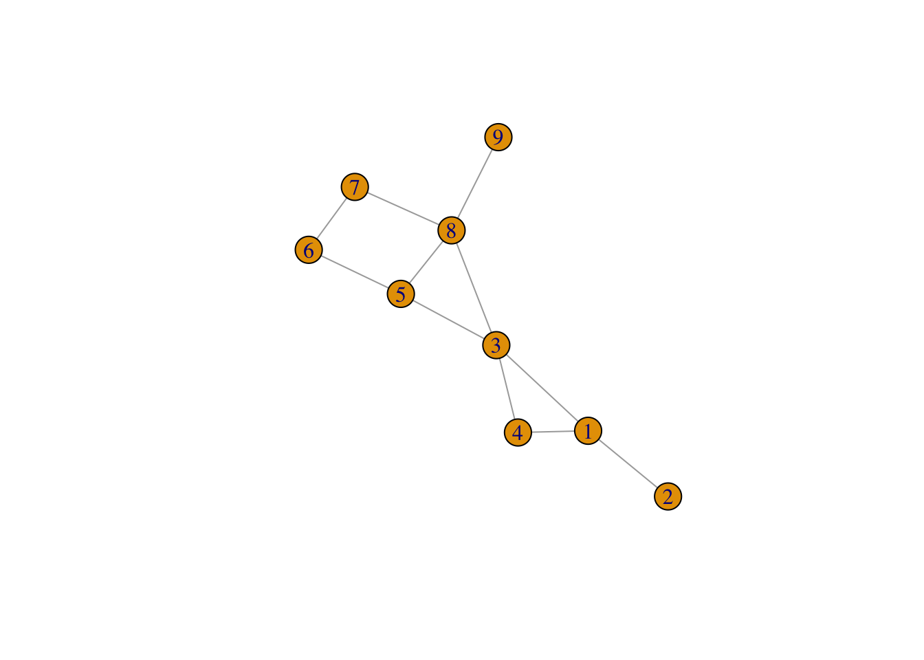
- We wish to create the following network in R. We do this by creating
two data frames,
nodesandlinks. Thenodesdata frame should contain two columns,id, which contains the names of the nodes, andtypewhich contains the type of each node. For now we shall have three types,A(nodes with id less than or equal to 4),B(nodes with id 8 or 9) andC- the rest.
The links data frame should contain four variables for
each edge in the graph. The four variables should be called
from, to, type, and
weight and should contain the name of the nodes (from and
to), the type (you can put in anything here for now as we will not use
it), and the weight. We will be using unweighted edges so set all edge
weights to 1.
library("igraph")
g <- graph_from_data_frame(links, vertices = nodes, directed = FALSE)
plot(g)
Make sure the graph you see corresponds to the graph you were supposed to enter.
Calculate the degree centrality scores of each node in the network. Use the
centr_degree()function to compute the degrees for each node. Recompute the graph density by hand and compare to the calculation done by R.Use the
A <- as_adjacency_matrix(g)to convert the graph to an adjacency matrix. What can you read from the matrix?If you multiply the adjacency matrix by itself,
A %*% A, then what will the resulting matrix tell you? What if you multiply the adjacency matrix by itself three times?Compute the average degree of the network, and the degree distribution. [Hint: you can use the
table()function for this last part. ]Compute the local, average, and global clustering coefficient. [Hint: use the
transitivity()function.]Compute the average shortest path and the betweenness [Hint: look at the
distances()andbetweenness()functions.]
Facebook data
Here we will try to run through the same steps as we did above but for a much larger network with information on social network data from facebook. The input-edges can be read as follows:
gg <- read_graph(url("https://biostatistics.dk/teaching/advtopicsB/download/facebook.txt"), directed = FALSE)Compute the network characteristics. Do you notice anything strange about the degree distribution? The input file contains a number of multiple edges. They can be removed using the
simplify()function on the graph.Identify the individuals that are “hubs” or “influencers” in the sense that they have many connections.
Look at the
closeness()function. It computes another feature of the graph that we haven’t talked about during the lectures. What does it compute?
Simulating networks
The igraph package has a number of functions for
simulating networks based on paramatric models.
Bernoulli random graphs are created with the functions
sample_gnp()orsample_gnm(). The difference between these two is that the first fixes the number of nodes and randomly draws edges with probabilityp, while the other fixes both the number of nodes and edges (but places the edges uniformly).Simulate a Bernoulli random graph with 1000 nodes and probability 1/1000. Plot the graph. Run some of the feature calculations on this graph - in particular
degree_distribution().Simulate another Bernoulli random graph with 1000 nodes but probability 1/100. Plot the graph. Run the same feature calculations on this graph - in particular
degree_distribution(). Note the difference? Why are they so substantially different?Now we will try to simulate other types of network and investigate how they induce different features. Consider trying the following functions:
sample_pa(n, power, directed=FALSE)Scale-free random graphsample_smallworld(1, 10, 2, 0.05)Watts-Strogatz random graph. (The first argument should be 1 to keep the dimension down)sample_sbm(n, pref.matrix, block.sizes)here,pref.matrixshould be a symmetric matrix giving the probability of an edge between pairs of states/types. The vectorblock.sizesgives the number of nodes of each type, and should sum ton.
Fitting models
- First we assume that the facebook data stemmed from a Bernoulli random graph. Estimate the edge probability if that were the case.
- Now we will fit the parameters from a scale-free model. Create a log-log plot based on a scale-free model and estimate the two parameters using linear regression.
- Try to estimate the same parameter using the
fit_power_law()function. - Simulate a scale-free model with the same parameters as estimated in the previous question. How does the simulated network characterisctics resemble the characteristics from the facebook data?
Testing models
- Pick a feature or two and test (using parametric bootstrap) whether the observed network is in accordance with the parametric model.
- Sample from the criterion that the degree sequence should be the
same as in the original data. Test whether that model is more flexible
and provides a different test for a feature of interest. [Hint: use
sample_degseq()]
Communities
The cluster_edge_betweenness() function derives clusters
based on the betweenness score, while the modularity()
function computes the modularity. The membership() function
extracts the group membership.
- Compute the communities for the initial simple data.
- Plot using
plot(cluster_edge_betweenness(g), g)wherecluster_edge_betweenness()is used to define the commmunities. What do you see? How is thecolargument defined (look at the help page for themembership()function) - Do the same for the facebook data.
2024