Day 4 solution overview
Principal component analysis
library("MASS")##
## Attaching package: 'MASS'## The following object is masked _by_ '.GlobalEnv':
##
## genotype## The following object is masked from 'package:dplyr':
##
## selectdata(biopsy)
names(biopsy)## [1] "ID" "V1" "V2" "V3" "V4" "V5" "V6" "V7" "V8"
## [10] "V9" "class"predictors <- biopsy[complete.cases(biopsy),2:10]
fit <- prcomp(predictors, scale=TRUE)
summary(fit)## Importance of components:
## PC1 PC2 PC3 PC4 PC5 PC6 PC7
## Standard deviation 2.4289 0.88088 0.73434 0.67796 0.61667 0.54943 0.54259
## Proportion of Variance 0.6555 0.08622 0.05992 0.05107 0.04225 0.03354 0.03271
## Cumulative Proportion 0.6555 0.74172 0.80163 0.85270 0.89496 0.92850 0.96121
## PC8 PC9
## Standard deviation 0.51062 0.29729
## Proportion of Variance 0.02897 0.00982
## Cumulative Proportion 0.99018 1.00000fit## Standard deviations (1, .., p=9):
## [1] 2.4288885 0.8808785 0.7343380 0.6779583 0.6166651 0.5494328 0.5425889
## [8] 0.5106230 0.2972932
##
## Rotation (n x k) = (9 x 9):
## PC1 PC2 PC3 PC4 PC5 PC6
## V1 -0.3020626 -0.14080053 0.866372452 -0.10782844 0.08032124 -0.24251752
## V2 -0.3807930 -0.04664031 -0.019937801 0.20425540 -0.14565287 -0.13903168
## V3 -0.3775825 -0.08242247 0.033510871 0.17586560 -0.10839155 -0.07452713
## V4 -0.3327236 -0.05209438 -0.412647341 -0.49317257 -0.01956898 -0.65462877
## V5 -0.3362340 0.16440439 -0.087742529 0.42738358 -0.63669325 0.06930891
## V6 -0.3350675 -0.26126062 0.000691478 -0.49861767 -0.12477294 0.60922054
## V7 -0.3457474 -0.22807676 -0.213071845 -0.01304734 0.22766572 0.29889733
## V8 -0.3355914 0.03396582 -0.134248356 0.41711347 0.69021015 0.02151820
## V9 -0.2302064 0.90555729 0.080492170 -0.25898781 0.10504168 0.14834515
## PC7 PC8 PC9
## V1 -0.008515668 0.24770729 -0.002747438
## V2 -0.205434260 -0.43629981 -0.733210938
## V3 -0.127209198 -0.58272674 0.667480798
## V4 0.123830400 0.16343403 0.046019211
## V5 0.211018210 0.45866910 0.066890623
## V6 0.402790095 -0.12665288 -0.076510293
## V7 -0.700417365 0.38371888 0.062241047
## V8 0.459782742 0.07401187 -0.022078692
## V9 -0.132116994 -0.05353693 0.007496101The
rotationelement is the interesting part.(and 3 + 4)
plot(fit)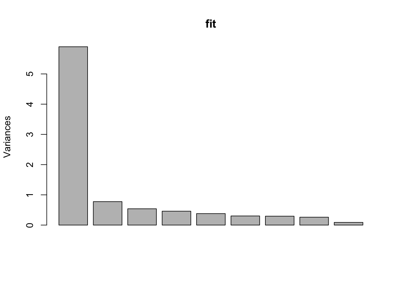
biplot(fit)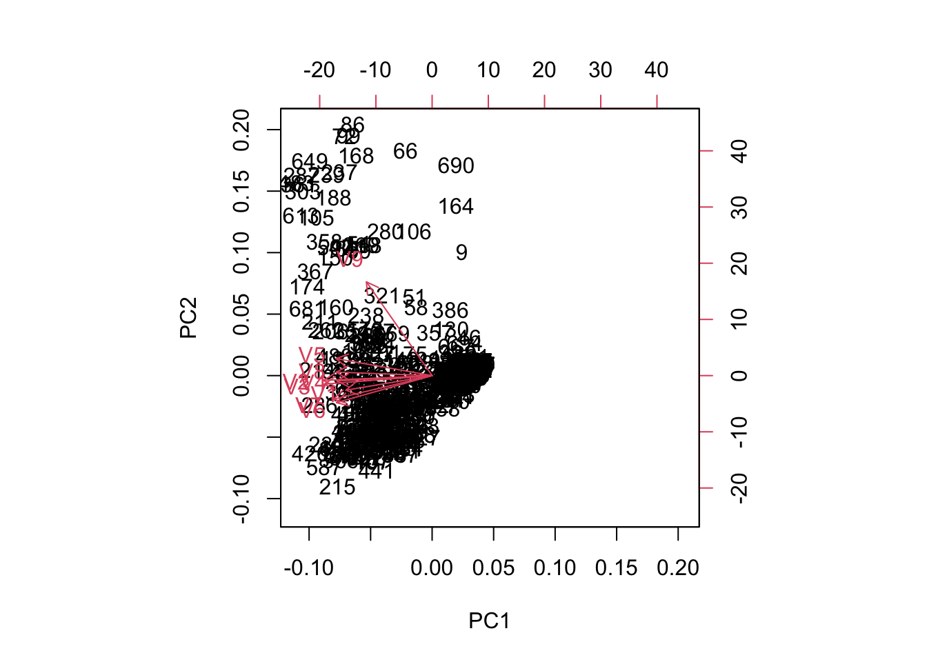
Only one real PC needed (from the elbow plot). The biplot shows that one variable drives PC2 while all of them have essentially the same effect on PC1. Not surprising as they are all more and more critical indicators of tumor features.
- Fitting using a formula model
fit2 <- prcomp(~ V1 + V2 + V3 + V3 + V5 + V6 + V7 + V8 + V9,
              data=biopsy, na.action=na.omit)
print(fit2)
## Standard deviations (1, .., p=8):
## [1] 6.6345189 2.2569305 1.9812100 1.7451112 1.5710111 1.3594598 1.2715023
## [8] 0.9005915
##
## Rotation (n x k) = (8 x 8):
## PC1 PC2 PC3 PC4 PC5 PC6
## V1 -0.3194268 -0.13885620 0.89523893 -0.25820349 0.021137857 -0.06694118
## V2 -0.4275683 0.22005419 0.01477139 0.41705715 0.153190217 0.17695828
## V3 -0.4170323 0.14900878 0.02785863 0.34835321 0.170043819 0.35841990
## V5 -0.2647245 0.19630122 -0.04734659 0.28691795 -0.350880265 -0.11400388
## V6 -0.4666288 -0.78704975 -0.31061644 -0.11865052 -0.191330240 0.11380645
## V7 -0.3073916 0.01185556 -0.16645553 0.02347393 0.442226055 -0.81713868
## V8 -0.3766912 0.46400242 -0.26454671 -0.73342853 0.009163472 0.17981165
## V9 -0.1304935 0.19149731 0.03370874 0.05635642 -0.769284716 -0.33127507
## PC7 PC8
## V1 -0.074256263 0.01103329
## V2 0.146717851 0.71992991
## V3 0.265037584 -0.67389149
## V5 -0.810922404 -0.11451718
## V6 -0.002565307 0.05180715
## V7 0.059128314 -0.10166461
## V8 -0.041837704 0.02713857
## V9 0.489761862 -0.02406411cor(predictors)## V1 V2 V3 V4 V5 V6 V7
## V1 1.0000000 0.6424815 0.6534700 0.4878287 0.5235960 0.5930914 0.5537424
## V2 0.6424815 1.0000000 0.9072282 0.7069770 0.7535440 0.6917088 0.7555592
## V3 0.6534700 0.9072282 1.0000000 0.6859481 0.7224624 0.7138775 0.7353435
## V4 0.4878287 0.7069770 0.6859481 1.0000000 0.5945478 0.6706483 0.6685671
## V5 0.5235960 0.7535440 0.7224624 0.5945478 1.0000000 0.5857161 0.6181279
## V6 0.5930914 0.6917088 0.7138775 0.6706483 0.5857161 1.0000000 0.6806149
## V7 0.5537424 0.7555592 0.7353435 0.6685671 0.6181279 0.6806149 1.0000000
## V8 0.5340659 0.7193460 0.7179634 0.6031211 0.6289264 0.5842802 0.6656015
## V9 0.3509572 0.4607547 0.4412576 0.4188983 0.4805833 0.3392104 0.3460109
## V8 V9
## V1 0.5340659 0.3509572
## V2 0.7193460 0.4607547
## V3 0.7179634 0.4412576
## V4 0.6031211 0.4188983
## V5 0.6289264 0.4805833
## V6 0.5842802 0.3392104
## V7 0.6656015 0.3460109
## V8 1.0000000 0.4337573
## V9 0.4337573 1.0000000Principal component regression
We already computed the PCs above so we can just use those. The
computed values can either be extracted as the x element or
by using the predict() function.
The outcome is binary so we will use a logistic regression model. Trying with the first four PCs.
y <- biopsy$class[complete.cases(biopsy)]
pcr <- glm(y ~ fit$x[,1] + fit$x[,2] + fit$x[,3] + fit$x[,4],
           family=binomial)
summary(pcr)
## ## Call: ## glm(formula = y ~ fit$x[, 1] + fit$x[, 2] + fit$x[, 3] + fit$x[, ## 4], family = binomial) ## ## Deviance Residuals: ## Min 1Q Median 3Q Max ## -3.1791 -0.1304 -0.0619 0.0228 2.4799 ## ## Coefficients: ## Estimate Std. Error z value Pr(>|z|) ## (Intercept) -1.0739 0.3035 -3.539 0.000402 *** ## fit$x[, 1] -2.4140 0.2556 -9.445 < 2e-16 *** ## fit$x[, 2] -0.1592 0.5050 -0.315 0.752540 ## fit$x[, 3] 0.7191 0.3273 2.197 0.028032 * ## fit$x[, 4] -0.9151 0.3691 -2.479 0.013159 * ## --- ## Signif. codes: 0 '***' 0.001 '**' 0.01 '*' 0.05 '.' 0.1 ' ' 1 ## ## (Dispersion parameter for binomial family taken to be 1) ## ## Null deviance: 884.35 on 682 degrees of freedom ## Residual deviance: 106.12 on 678 degrees of freedom ## AIC: 116.12 ## ## Number of Fisher Scoring iterations: 8PC 1 provides a lot of info about the outcome, and the coefficient is negative which means that at increase for the PC value will lower the odds of a malignant outcome. However, recall that the rotation matrix for the first principal component only had negative weights so when that is combined we get that an increase in any predictor will result in an increase in log odds of a malignant tumor.
We also see that even though the PCs are ranked from highest variation to lowest variation their p-values are not necessarily ranked in the same order.Primarily prediction as the components are difficult to interpret.
pcr2 <- glm(y ~ fit$x[,1] + fit$x[,2],
           family=binomial)
summary(pcr2)
## ## Call: ## glm(formula = y ~ fit$x[, 1] + fit$x[, 2], family = binomial) ## ## Deviance Residuals: ## Min 1Q Median 3Q Max ## -3.05575 -0.13442 -0.09243 0.02699 2.76606 ## ## Coefficients: ## Estimate Std. Error z value Pr(>|z|) ## (Intercept) -0.9436 0.2636 -3.579 0.000345 *** ## fit$x[, 1] -2.3060 0.2197 -10.496 < 2e-16 *** ## fit$x[, 2] -0.1815 0.3225 -0.563 0.573455 ## --- ## Signif. codes: 0 '***' 0.001 '**' 0.01 '*' 0.05 '.' 0.1 ' ' 1 ## ## (Dispersion parameter for binomial family taken to be 1) ## ## Null deviance: 884.35 on 682 degrees of freedom ## Residual deviance: 119.37 on 680 degrees of freedom ## AIC: 125.37 ## ## Number of Fisher Scoring iterations: 8We see that there is hardly any difference for the predictors. The reason why the predictors are not completely identical to the fit above where we had 4 predictors is because of the non-identity link function.
We will need to see how the predictability improves with number of components.
GWAS analysis
First we get the data
options(timeout = 5*60)
load(url("https://www.biostatistics.dk/teaching/bioinformatics/data/gwasgt.rda"))
load(url("https://www.biostatistics.dk/teaching/bioinformatics/data/gwaspt.rda"))- The number of columns in the
genotypedataframe shows the number of SNPs available.
dim(genotypes)## [1] 1324 32019If we had just a single SNP available we would start by doing a multiple linear regression analysis since the phenotype outcome (BMI) is quantitative. That would also allow us to adjust for the other variables that are available in the
phenotypesdataframe.For example (just using the 1st column in
genotypes) as my one SNP:
m1 <- lm(BMI ~ genotypes[,1] + gender + age, data=phenotypes)
summary(m1)
##
## Call:
## lm(formula = BMI ~ genotypes[, 1] + gender + age, data = phenotypes)
##
## Residuals:
## Min 1Q Median 3Q Max
## -3.2233 -0.7367 0.0005 0.7372 3.5467
##
## Coefficients:
## Estimate Std. Error t value Pr(>|t|)
## (Intercept) 22.393689 0.163467 136.992 < 2e-16 ***
## genotypes[, 1] -0.182344 0.066560 -2.740 0.00624 **
## genderMale 1.148445 0.058668 19.575 < 2e-16 ***
## age 0.002363 0.005983 0.395 0.69295
## ---
## Signif. codes: 0 '***' 0.001 '**' 0.01 '*' 0.05 '.' 0.1 ' ' 1
##
## Residual standard error: 1.067 on 1320 degrees of freedom
## Multiple R-squared: 0.228, Adjusted R-squared: 0.2262
## F-statistic: 129.9 on 3 and 1320 DF, p-value: < 2.2e-16In the following we are discarding
ageandgendersince the function we will be using only takes a single matrix of predictors. We could include their effects indirectly by subtracting their respective (estimated) effects fromBMIand analysing the residuals as outcomes instead.library("MESS") full <- mfastLmCpp(phenotypes$BMI, genotypes)For the Manhattan plot we use that the 3rd column in
fullis the t test statistic and we know there are 1324 rows.logpvals <- -log10(2*pt(-abs(full[,3]), df=1324-2)) plot(logpvals, col=(seq(32019)>11283)+1)
Now running lasso
library("glmnet")
l1 <- glmnet(genotypes, phenotypes$BMI)
l12 <- cv.glmnet(genotypes, phenotypes$BMI) # Get the lambda parameter
We can check if the predictors selected are the same for the two methods.
estcoefs <- coef(l1, s=l12$lambda.1se)
pick <- rownames(estcoefs)[as.numeric(estcoefs) != 0]  # Remove the intercept
pick
## [1] "(Intercept)" "V802" "V2551" "V4093" "V4624" ## [6] "V4683" "V21163" "V31141"The previous analysis produced this set
seq(NROW(full))[logpvals > -log10(0.05/NCOL(genotypes))]## [1] 21163 31141Same as above with
alphaparameter set.For computing the genomic controls we find the median of the \(p\)-values
median(full[,3]^2)## [1] 0.4544575Since this number is klower than the default level of 0.456 there is no need for correcting for genomic controls.
Population admixture
Because hidden population admixture may act as a confounder between allele frequencies and the outcome and may mask the true relationship.
Using the
onlinePCApackage for fast computation of the first principal components.library("onlinePCA")## Loading required package: RSpectraadmixturepca <- batchpca(genotypes, q=1)Let’s extract the effect of the PC
am1 <- lm(phenotypes$BMI ~ admixturepca$vectors)
coef(am1)
## (Intercept) admixturepca$vectors ## 25.68605 98.24532summary(am1)## ## Call: ## lm(formula = phenotypes$BMI ~ admixturepca$vectors) ## ## Residuals: ## Min 1Q Median 3Q Max ## -3.7503 -0.8594 0.0103 0.8569 4.1692 ## ## Coefficients: ## Estimate Std. Error t value Pr(>|t|) ## (Intercept) 25.686 3.672 6.996 4.18e-12 *** ## admixturepca$vectors 98.245 133.599 0.735 0.462 ## --- ## Signif. codes: 0 '***' 0.001 '**' 0.01 '*' 0.05 '.' 0.1 ' ' 1 ## ## Residual standard error: 1.213 on 1322 degrees of freedom ## Multiple R-squared: 0.0004089, Adjusted R-squared: -0.0003472 ## F-statistic: 0.5408 on 1 and 1322 DF, p-value: 0.4622adjustedBMI <- phenotypes$BMI-coef(am1)[2]*admixturepca$vectors # Subtracting the effect full2 <- mfastLmCpp(adjustedBMI, genotypes) logpvals <- -log10(2*pt(-abs(full2[,3]), df=1324-3)) plot(logpvals, col=(seq(32019)>11283)+1)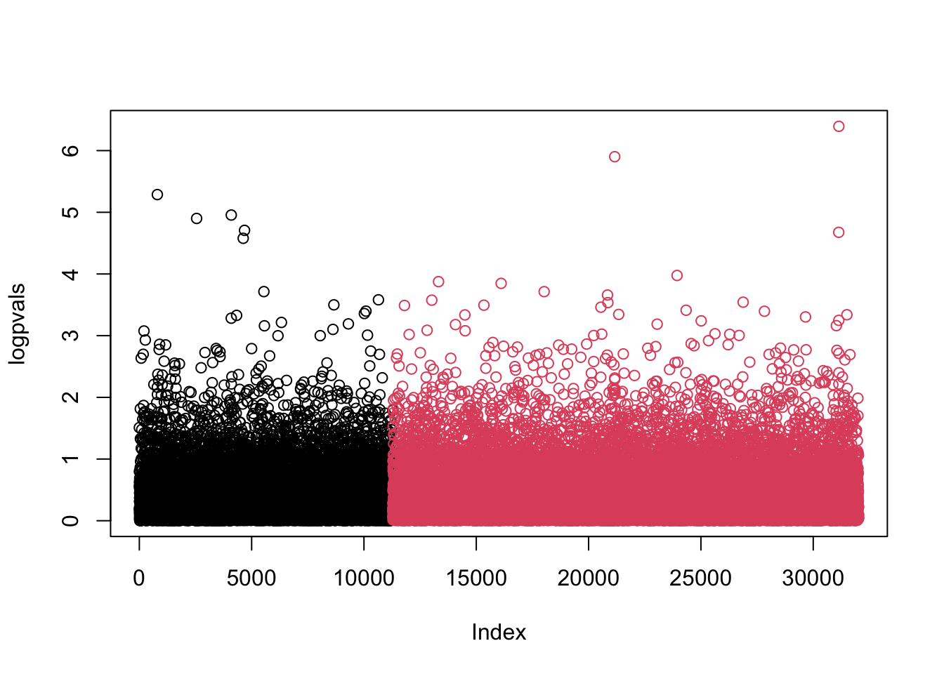
If at all possible we should use SNPs that are not our primary SNPs of interest.
Hertability
The minor allele frequencies are
MAF <- colMeans(genotypes)/2 # Minor allele frequencies
MAF[MAF>.5] <- 1-MAF[MAF>.5]
Compute the SDs for each column
sds <- sqrt(2*MAF*(1-MAF))Running the code
W <- t((t(genotypes) - 2*MAF)/sqrt(2*MAF*(1-MAF)))
y <- phenotypes$BMI
N <- length(y)
A <- tcrossprod(W) / ncol(genotypes)
library("coxme")
## Loading required package: survival## Loading required package: bdsmatrix## ## Attaching package: 'bdsmatrix'## The following object is masked from 'package:base': ## ## backsolveid <- 1:N res <- lmekin(y ~ 1 + (1|id), varlist=list(id=A)) res## Linear mixed-effects kinship model fit by maximum likelihood ## Data: NULL ## Log-likelihood = -2133.487 ## n= 1324 ## ## ## Model: y ~ 1 + (1 | id) ## Fixed coefficients ## Value Std Error z p ## (Intercept) 22.98614 0.03063669 750.28 0 ## ## Random effects ## Group Variable Std Dev Variance ## id id 0.4770917 0.2276165 ## Residual error= 1.114754We are computing the SNP heritability. The
Amatrix contains the correlation structure derived from the SNPs.The SNP heritability is
0.2276165 / (0.2276165 + 1.114715^2)## [1] 0.1548195
Correlation
pick <- 791:810
library("energy")
p.cor <- cor(genotypes[,pick])
p.cor
## [,1] [,2] [,3] [,4] [,5]
## [1,] 1.000000000 -0.012669801 -0.048396339 4.370489e-02 0.032610592
## [2,] -0.012669801 1.000000000 0.009076470 6.367929e-02 0.006451871
## [3,] -0.048396339 0.009076470 1.000000000 1.990846e-03 -0.009414619
## [4,] 0.043704888 0.063679292 0.001990846 1.000000e+00 0.021740447
## [5,] 0.032610592 0.006451871 -0.009414619 2.174045e-02 1.000000000
## [6,] 0.014852508 -0.006774466 0.026906778 -2.267627e-02 -0.012128030
## [7,] 0.020488031 0.004057904 0.001195557 3.757981e-03 -0.024954324
## [8,] 0.031114192 -0.033951167 -0.001505205 -2.580557e-02 -0.055412127
## [9,] 0.005569970 -0.019096029 0.040142955 -9.999918e-03 0.005434349
## [10,] 0.029969416 0.013594396 0.029471316 -1.600414e-02 0.069466388
## [11,] 0.016083105 -0.017543667 0.034330641 3.548986e-02 0.018649033
## [12,] 0.022026977 0.033646352 -0.020784142 1.133123e-02 0.008320726
## [13,] -0.031168491 0.019540373 0.027955360 5.953349e-02 0.032280868
## [14,] 0.009883652 0.013219369 0.008875035 -1.806378e-03 0.014885166
## [15,] -0.033923864 0.005761538 -0.001628895 7.373480e-03 -0.031941876
## [16,] -0.021362275 0.029971076 0.017698330 -7.970986e-03 -0.008556213
## [17,] -0.031674426 -0.007735149 0.017223823 -1.171268e-02 -0.003185612
## [18,] -0.043510060 -0.001906256 0.002638056 -3.199698e-02 0.025748241
## [19,] 0.004365961 0.021260386 -0.023098832 2.217117e-02 0.024520975
## [20,] -0.003384732 -0.003379811 0.016764175 1.240761e-05 -0.022672361
## [,6] [,7] [,8] [,9] [,10]
## [1,] 0.014852508 0.020488031 0.031114192 0.005569970 0.029969416
## [2,] -0.006774466 0.004057904 -0.033951167 -0.019096029 0.013594396
## [3,] 0.026906778 0.001195557 -0.001505205 0.040142955 0.029471316
## [4,] -0.022676274 0.003757981 -0.025805572 -0.009999918 -0.016004142
## [5,] -0.012128030 -0.024954324 -0.055412127 0.005434349 0.069466388
## [6,] 1.000000000 -0.009209339 -0.002980107 0.001919025 -0.039495777
## [7,] -0.009209339 1.000000000 0.184684950 0.125033108 0.200841299
## [8,] -0.002980107 0.184684950 1.000000000 0.182352384 0.248065311
## [9,] 0.001919025 0.125033108 0.182352384 1.000000000 0.197987411
## [10,] -0.039495777 0.200841299 0.248065311 0.197987411 1.000000000
## [11,] 0.052129891 0.098559134 0.177560389 0.077129174 0.173679275
## [12,] -0.004151115 0.313348052 0.480591392 0.289747633 0.563915687
## [13,] -0.022597884 0.103736946 0.164538357 0.044536789 0.163469497
## [14,] 0.022654566 0.111493202 0.128216289 0.082938269 0.179095036
## [15,] 0.034796899 0.162604344 0.245357249 0.141665912 0.289854195
## [16,] 0.007477150 0.061227557 0.139044339 0.053129858 0.156760885
## [17,] -0.026413678 0.183071512 0.179466362 0.129050005 0.221617346
## [18,] -0.012594110 -0.001209319 -0.039820649 -0.029573594 0.014785367
## [19,] -0.035070434 0.003129502 -0.013357642 -0.026508145 -0.004121673
## [20,] -0.005206238 0.022172940 0.001500433 -0.019341256 -0.029487753
## [,11] [,12] [,13] [,14] [,15]
## [1,] 0.016083105 0.022026977 -0.03116849 0.009883652 -0.033923864
## [2,] -0.017543667 0.033646352 0.01954037 0.013219369 0.005761538
## [3,] 0.034330641 -0.020784142 0.02795536 0.008875035 -0.001628895
## [4,] 0.035489864 0.011331228 0.05953349 -0.001806378 0.007373480
## [5,] 0.018649033 0.008320726 0.03228087 0.014885166 -0.031941876
## [6,] 0.052129891 -0.004151115 -0.02259788 0.022654566 0.034796899
## [7,] 0.098559134 0.313348052 0.10373695 0.111493202 0.162604344
## [8,] 0.177560389 0.480591392 0.16453836 0.128216289 0.245357249
## [9,] 0.077129174 0.289747633 0.04453679 0.082938269 0.141665912
## [10,] 0.173679275 0.563915687 0.16346950 0.179095036 0.289854195
## [11,] 1.000000000 0.351410659 0.15601727 0.081090594 0.208183515
## [12,] 0.351410659 1.000000000 0.30305809 0.312783793 0.499459848
## [13,] 0.156017266 0.303058093 1.00000000 0.083721672 0.177005709
## [14,] 0.081090594 0.312783793 0.08372167 1.000000000 0.183558250
## [15,] 0.208183515 0.499459848 0.17700571 0.183558250 1.000000000
## [16,] 0.059870362 0.244830350 0.04873371 0.080799784 0.130202752
## [17,] 0.116762097 0.388851186 0.09872636 0.137842185 0.179302359
## [18,] -0.028608050 0.005914917 -0.04950697 0.022330622 -0.016048450
## [19,] -0.004382413 -0.016199626 -0.01830547 -0.002094196 -0.018029261
## [20,] 0.035848085 -0.007354626 0.02443749 -0.009528773 -0.034465146
## [,16] [,17] [,18] [,19] [,20]
## [1,] -0.021362275 -0.031674426 -0.043510060 0.004365961 -3.384732e-03
## [2,] 0.029971076 -0.007735149 -0.001906256 0.021260386 -3.379811e-03
## [3,] 0.017698330 0.017223823 0.002638056 -0.023098832 1.676418e-02
## [4,] -0.007970986 -0.011712681 -0.031996978 0.022171167 1.240761e-05
## [5,] -0.008556213 -0.003185612 0.025748241 0.024520975 -2.267236e-02
## [6,] 0.007477150 -0.026413678 -0.012594110 -0.035070434 -5.206238e-03
## [7,] 0.061227557 0.183071512 -0.001209319 0.003129502 2.217294e-02
## [8,] 0.139044339 0.179466362 -0.039820649 -0.013357642 1.500433e-03
## [9,] 0.053129858 0.129050005 -0.029573594 -0.026508145 -1.934126e-02
## [10,] 0.156760885 0.221617346 0.014785367 -0.004121673 -2.948775e-02
## [11,] 0.059870362 0.116762097 -0.028608050 -0.004382413 3.584809e-02
## [12,] 0.244830350 0.388851186 0.005914917 -0.016199626 -7.354626e-03
## [13,] 0.048733707 0.098726363 -0.049506973 -0.018305466 2.443749e-02
## [14,] 0.080799784 0.137842185 0.022330622 -0.002094196 -9.528773e-03
## [15,] 0.130202752 0.179302359 -0.016048450 -0.018029261 -3.446515e-02
## [16,] 1.000000000 0.093936474 0.035813752 -0.036423989 -5.274574e-02
## [17,] 0.093936474 1.000000000 0.024919247 0.005618310 2.956952e-03
## [18,] 0.035813752 0.024919247 1.000000000 -0.041379204 -4.839268e-02
## [19,] -0.036423989 0.005618310 -0.041379204 1.000000000 5.509289e-03
## [20,] -0.052745737 0.002956952 -0.048392675 0.005509289 1.000000e+00sapply(791:810, function(i) { dcor(genotypes[,802], genotypes[,i])})## [1] 0.018188657 0.028086472 0.016514448 0.020326953 0.019355364 0.004539388
## [7] 0.342693860 0.478482932 0.335991847 0.563204196 0.361703514 1.000000000
## [13] 0.361223935 0.359625881 0.514324052 0.296790709 0.408933458 0.023455655
## [19] 0.015190565 0.009542506dcor(genotypes[,802], phenotypes$BMI)## [1] 0.1304523dcorT.test(genotypes[,802], phenotypes$BMI)##
## dcor t-test of independence for high dimension
##
## data: genotypes[, 802] and phenotypes$BMI
## T = 14.709, df = 874501, p-value < 2.2e-16
## sample estimates:
## Bias corrected dcor
## 0.0157272library("pscl")
load(url("http://www.biostatistics.dk/microbiome.rda"))
head(microbiome, 50)
z1 <- zeroinfl(round(value) ~ condition + gender + age,
subset=(otu==1), data=microbiome)
summary(z1)
exp(0.26)
z2 <- zeroinfl(round(value) ~ condition + gender + age,
dist="negbin",
subset=(otu==1), data=microbiome)
summary(z2)
z3 <- zeroinfl(round(value) ~ condition + gender + age |
gender,
subset=(otu==1), data=microbiome)
summary(z3) Claus Ekstrøm 2023