Day 1 solution overview
Multiple testing
Out of 21500 test we’d expect around
0.05*21500to be significant by chance.(and 3, 5 and 6)
library("MESS")
data(superroot2)

pval <- by(superroot2,
           superroot2$gene,
           FUN=function(dat) {
              anova(lm(log(signal) ~ array + color + plant,
                       data=dat))[3,5]} )

library("ggplot2")
library("tidyverse")
DF <- data.frame(pval=as.vector(pval))

DF %>% ggplot(aes(x=pval)) + geom_histogram(col="lightblue")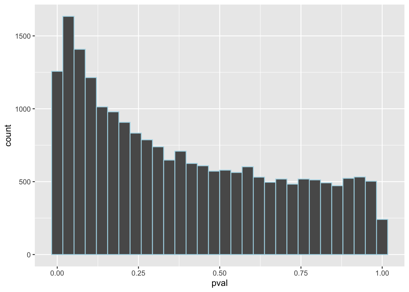
# Remember that some are missing

p1 <- p.adjust(as.vector(pval), method="bonferroni")
p2 <- p.adjust(as.vector(pval), method="holm")
p3 <- p.adjust(as.vector(pval), method="BH") # FDR

head(sort(pval))
## superroot2$gene
## AT3G59930.1 AT2G39350.1 AT3G60140.1 AT4G19030.1 AT4G31500.1 AT5G13910.1
## 1.048266e-05 1.781166e-05 2.880092e-05 3.298942e-05 3.410671e-05 3.438769e-05head(sort(p1))## [1] 0.2253667 0.3829328 0.6191910 0.7092394 0.7332602 0.7393009head(sort(p2))## [1] 0.2253667 0.3829150 0.6191334 0.7091405 0.7331238 0.7391290head(sort(p3))## [1] 0.1075944 0.1075944 0.1075944 0.1075944 0.1075944 0.1075944Note that one of the tests resulted in a
NAso there are actually only 21499 tests undertaken. If this number is used as the denominator then the numbers match.Due to the nature of the BH approach. If an earlier p-value had a lower adjusted fdr-value then that value is used for lower ranked adjusted fdr values.
Penalized regression
library("glmnet")
load(url("http://www.biostatistics.dk/teaching/advtopicsA/data/lassodata.rda"))

m1 <- glmnet(genotype, phenotype)
Ensure that the penalty is the same across predictors such that it does not depend on scale.
m2 <- cv.glmnet(genotype, phenotype)
plot(m2)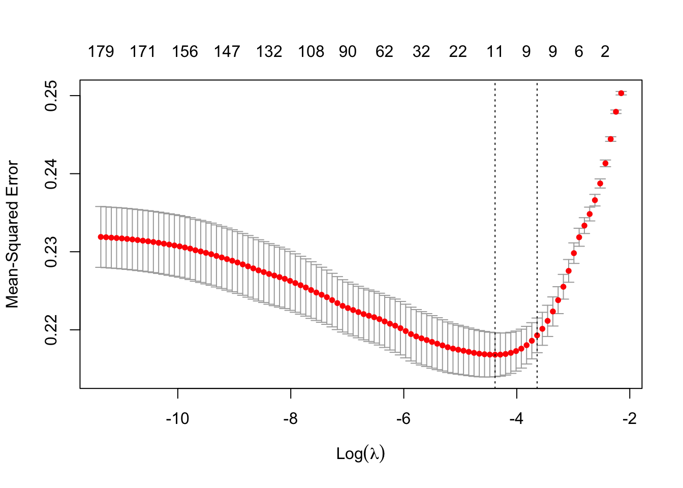
lambda <- m2$lambda.1seests <- coef(m1, s=lambda)
ests[ests != 0]## <sparse>[ <logic> ]: .M.sub.i.logical() maybe inefficient## [1] 6.155399e-01 7.945800e-02 -1.511681e-01 4.578236e-14 -2.143880e-02
## [6] 1.214096e-01 -1.767616e-02 1.371258e-01 1.326876e-01 1.127302e-03m3 <- glmnet(genotype, phenotype, family="binomial")
m4 <- cv.glmnet(genotype, phenotype, family="binomial")
plot(m3)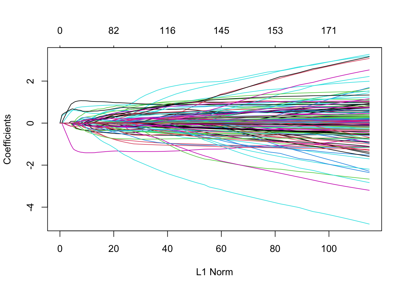
plot(m4)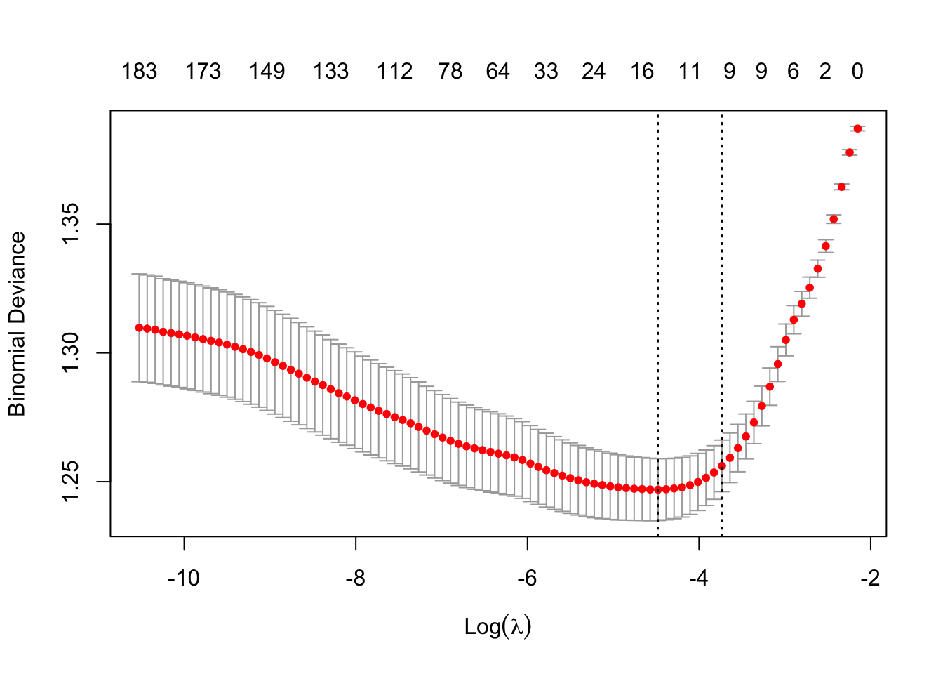
ests2 <- coef(m3, s=m4$lambda.1se)
ests2[ests2 != 0]
## <sparse>[ <logic> ]: .M.sub.i.logical() maybe inefficient## [1] 6.062753e-01 3.685309e-01 -7.083144e-01 7.122772e-14 -1.027700e-01
## [6] 5.261112e-01 -8.621539e-02 6.335221e-01 5.779711e-01 7.274392e-03m5 <- glmnet(genotype, phenotype, alpha=0, family="binomial")
m6 <- cv.glmnet(genotype, phenotype, alpha=0, family="binomial")
plot(m5)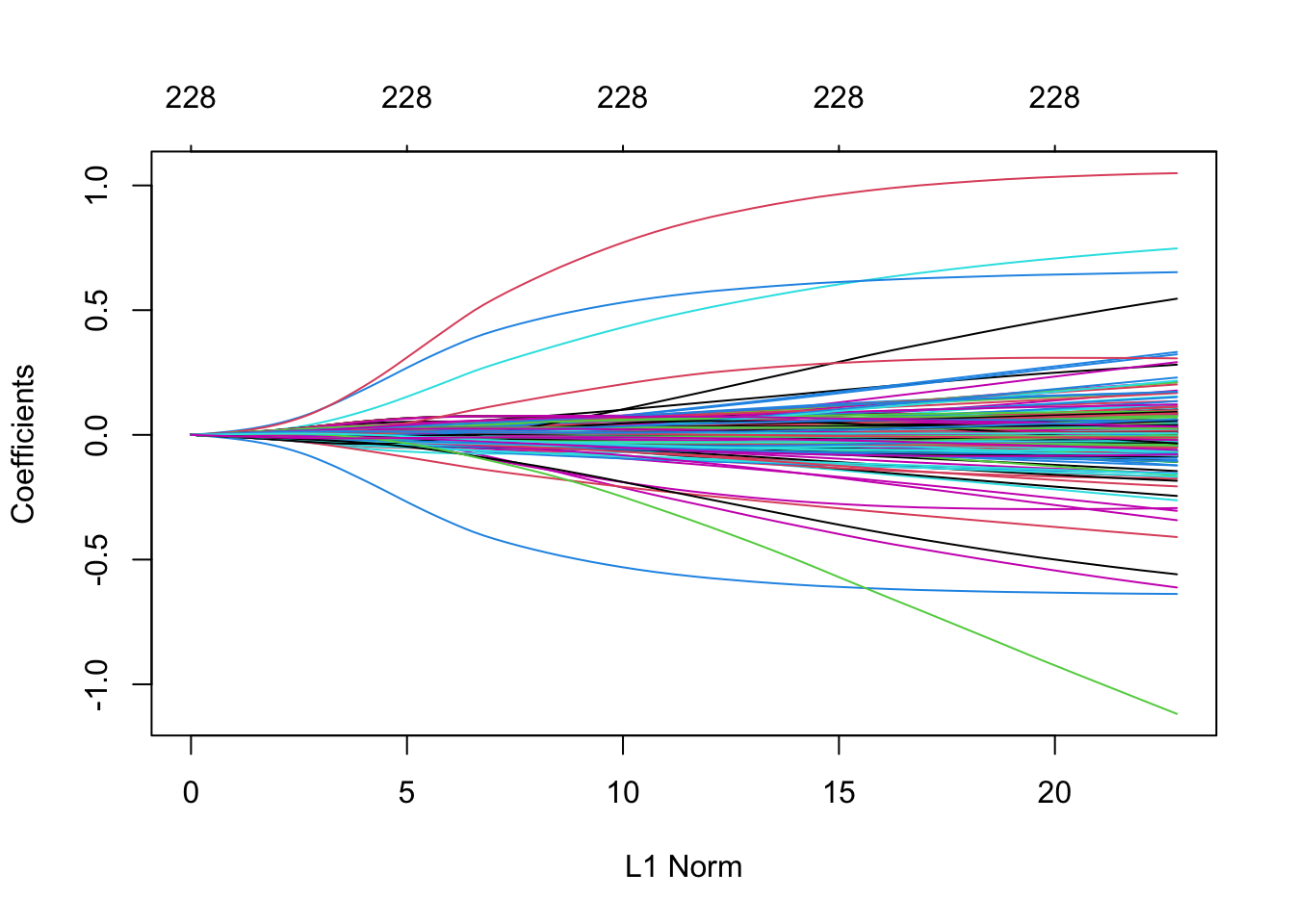
plot(m6)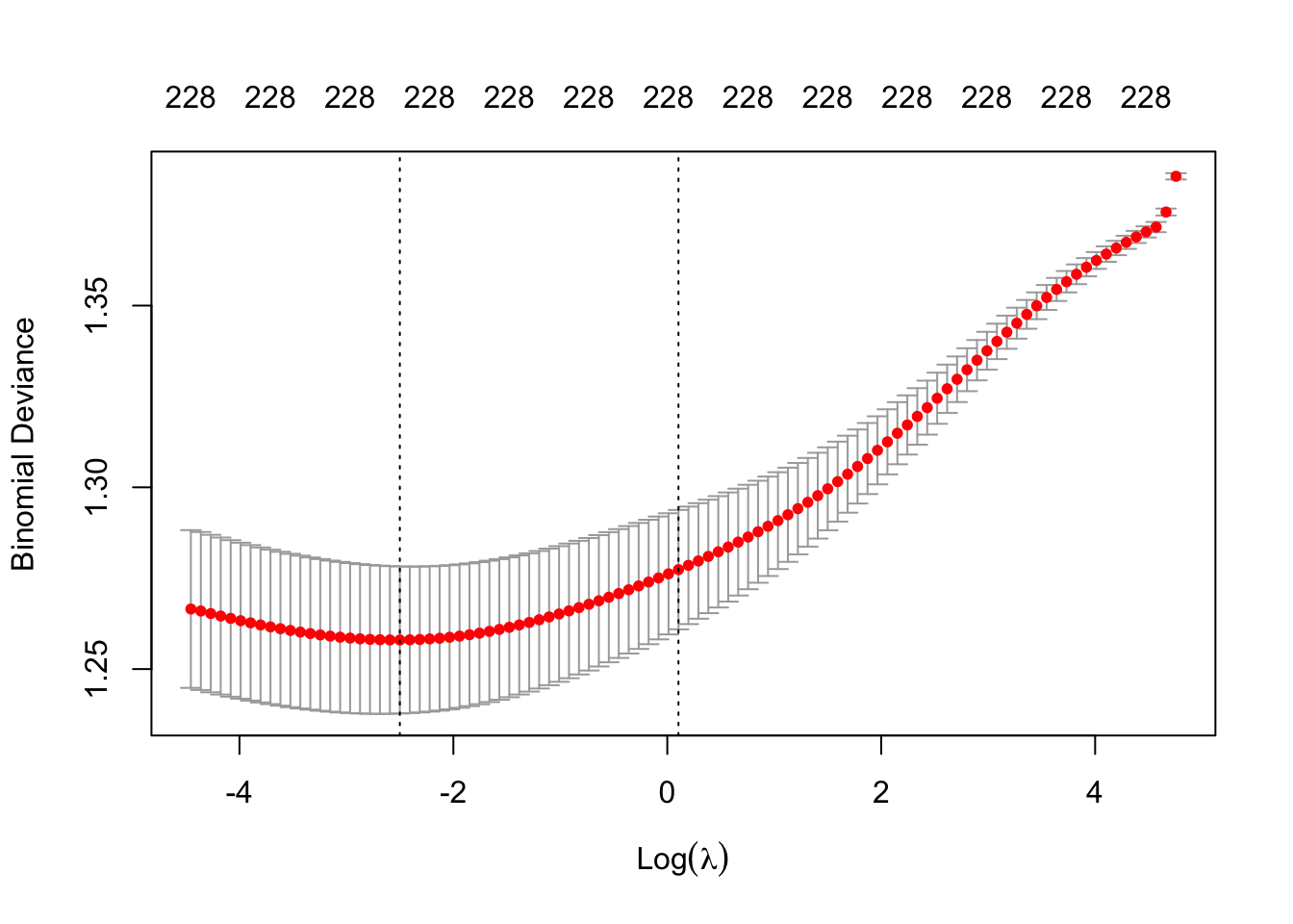
ests2 <- coef(m5, s=m6$lambda.1se) # Gets them all since none are zerom7 <- glmnet(genotype, phenotype, alpha=.67, family="binomial")
m8 <- cv.glmnet(genotype, phenotype, alpha=.67, family="binomial")
plot(m7)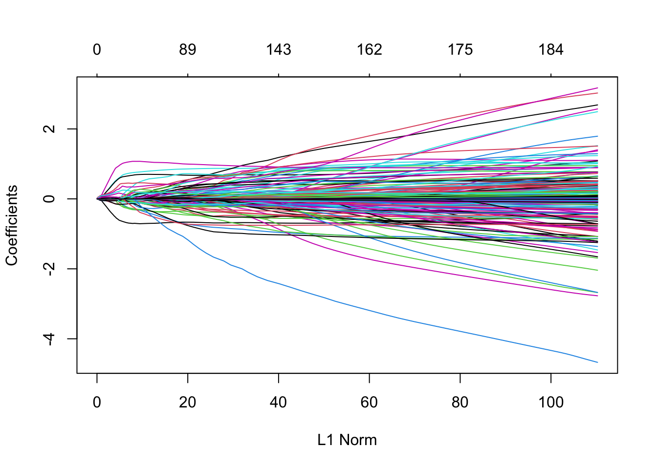
plot(m8)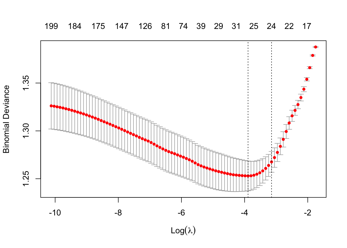
ests2 <- coef(m7, s=m8$lambda.1se)
ests2[ests2 != 0]
## <sparse>[ <logic> ]: .M.sub.i.logical() maybe inefficient## [1] 0.380817195 0.276653411 -0.298172779 0.270867271 -0.076465628
## [6] -0.006182403 0.169990524 0.041253335 0.040144873 0.006350749
## [11] 0.038004138 -0.024572992 -0.023649148 0.095457931 -0.021923444
## [16] -0.021274718 -0.064163458 0.502432620 0.141833575 0.059611682
## [21] -0.058574656 -0.057528482 0.121862616 0.056408785 -0.055123872Claus Ekstrøm 2023